Assembly x86 programming 101 : chapter 7, ASCII Mandelbrot

Although we already covered numerous basics in x86 assembly so far, one thing that has not been discussed yet is the use of floating point computation : namely numbers with a decimal part. However when working with computers, we love integers 🥰! No rounding, no loss of precision, no absorption problems, etc.. Unfortunately, non-integer values arise in many real world problems hence it is rather useful to know a little bit about them.

In this post, we will write a program that draws an ASCII version of the Mandelbrot set. The Mandelbrot set is a famous fractal that has been intensively rendered on computers in all of its shapes : with colors, in 3d, etc.. Its computation however relies on complex numbers arithmetic, it is hence necessary to manipulate floating point numbers 🏄. We will see here how to draw an ASCII version of this fractal by relying on some basic floating point number operations in assembly.

More on branching

Before diving into the world of floating points numbers, let’s add some details about branching in x86 assembly. We have already used testing operations such as cmp and test in the previous chapters. These were useful to write conditionals and loops thanks to branching instructions like jge.

Signed comparisons

There are however other branching instructions that we did not cover, such as jbe (jump if bellow or equal) or ja (jump above). The reason why several instructions exist is that some of them perform signed comparisons.

Internally, the use of the comparison instructions such as cmp and test set internal flags that dictate the behavior of the branching instructions. To see that in practice, let’s create a simple example :

1
2
3
4
5
6
7
8
9
10
11
12
13
14
15
16
17
18
19
mov al, 43
mov bl, 42

cmp al, bl
jle .L_endif

; if_no_jump

    ; printing
    xor eax, eax
    lea rdi, [jumping_str]
    call printf

.L_endif:

; [...]

branching_str:
    .asciz "not jumping!\n"

This code performs a comparison of the two 1-byte registers al and bl and then prints 🖨️ a string if the value in the first register al is lower or equal to the value in the second register bl. If you test this program, you should observe that the comparison is not verified since 43 > 42, hence the string is printed to the terminal.

Now, let’s replace the value 43 by the value 150 : mov al, 150. You will observe that the program now skips the printing instructions! 😱

The reason why is that the jle instruction performs a signed comparison. Indeed, depending on wether the values are signed or not, they are not interpreted the same way. Let’s run the program in gdb and add a breakpoint after the mov instructions. If we print the al value withp $al, we should get : 1 = -106! We can see that by default, the p command interprets the value as signed.

We can then use the command p/u $al that outputs 150 : this time the value is interpreted as being unsigned. As our value is coded on 1 byte, or 8 bits, the unsigned version can code values between 0 and 255 and the signed version will however represent values between -128 and 127. You can replace the value 150 in our code by -106 and see that it has no effect as the binary code is the same!

Now we can replace the jle instruction with jbe. Still with the value 150 for al, the program should now execute the printing operations as the jbe instruction performs an unsigned comparaison, and correctly interprets the value as 150 👌.

Flags registers

Internally, the comparison instructions and the conditional branching instructions are connected through the flags register. These flags are internally set by the comparison instructions and their values will act on the behavior of the jumps.

We will test it in GDB by re-setting the comparison instruction to jle in our code, in order to make the program jump. We can then add a breakpoint to pause the program just before the jle instruction. The p $eflags command can give us information about the flags that are set to 1 : $1 = [ PF AF IF OF ]. We can look at this page for instance to verify when the jump occurs with jle. We can see that it can happen when SF (the sign flag) is different than OF (the overflow flag), which is the case here as OF is set to 1 but not SF.

On the other hand, we can see on the page that a jump occurs with the jbe instruction when CF=1 or ZF=1. If we modify our program again to set al to 41 and bl to b42, we can see that the jump occurs with jbe. If we print the $eflags register as previously we obtain : $1 = [ CF PF AF SF IF ]. We can see that CF (carry flag) is set to 1, which triggers the jump.

Floating point operations in x86 assembly

Manipulating non-integer numbers is a whole new world in assembly programming. Indeed, these numbers are coded as “floating points” (floats for short), meaning the bits that code them are decomposed into 2 parts : the mantissa and the exponent. The mantissa is an integer that is to be multiplied (scaled) by a negative power, hence the exponent. Usually, as numbers are coded in binary, the base 2 is used for the exponent.

Floating points operations in processors are performed by a dedicated component called the Floating Point Unit (FPU). Hence, the assembly arithmetic instructions are completely separated from their analog integer ones.

How are floats implemented in C ?

One possible source of inspiration to see how we can perform theses operations is to look at the assembly codes automatically generated from a C code that performs floating pointes operations. Let’s start with a simple example :

1
2
3
4
5
6
7
8
9
10
11
#include <stdlib.h>
#include <stdio.h>

int main(int argc, char* argv[]) {

    double nbf = 0.25;
    nbf = nbf * 0.5;
    printf("result: %f\n", nbf);

    return 0;
}

You can compile with GCC and run this program to verify that the printed value is 0.125. In thi example, we work with double precision floating point numbers, meaning these numbers are coded on 8 bytes.

We can now use GCC to produce x86 assembly code from this C program with the following command : gcc -S floating_points.c -masm=intel -fdiagnostics-color=always -fverbose-asm -o floating_points.s. This command allows to create an assembly source file by using the same syntax as the one we employ, and by adding useful annotations regarding the original C code.

Without going into all the details of the resulting file, we can have a look at the sections where the comments refer to the 3 lines of our main function :

1
2
3
4
5
6
7
8
9
10
11
12
13
14
15
16
17
18
19
20
; floating_points.c:9:     double nbfd = 0.25;
    .loc 1 9 12
    movsd	xmm0, QWORD PTR .LC0[rip]	; tmp84,
    movsd	QWORD PTR -8[rbp], xmm0	; nbfd, tmp84

; floating_points.c:10:     nbfd = nbfd * 0.5;
    .loc 1 10 10
    movsd	xmm1, QWORD PTR -8[rbp]	; tmp86, nbfd
    movsd	xmm0, QWORD PTR .LC1[rip]	; tmp87,
    mulsd	xmm0, xmm1	; tmp85, tmp86
    movsd	QWORD PTR -8[rbp], xmm0	; nbfd, tmp85

; floating_points.c:11:     printf("result: %f\n", nbfd);
    .loc 1 11 5
    mov	rax, QWORD PTR -8[rbp]	; tmp88, nbfd
    movq	xmm0, rax	;, tmp88
    lea	rax, .LC2[rip]	; tmp89,
    mov	rdi, rax	;, tmp89
    mov	eax, 1	;,
    call	printf@PLT	;

Vector registers and arithmetic operations

Let’s focus on the first part of the code, that consists in loading the value 0.25 in the variable. We see a new kind of register here : xmm0.

This register is actually part of a set of registers called vector registers. These are employed for high performances floating point operations as they allow to perform the same operation on multiple floating point values at the same time! In this chapter however, we will only use them sequentially.

We can see that the content of these registers can be stored in memory as we would do for other registers with the dedicated operation movsd. In this case, as we declared a double variable in our C code, the value will be manipulated as a 8 bytes value (double precision).

If we now look at the next lines of the generated assembly code, we can see the an example of the floating point multiplication ✖️ with the mulsd operation (for 8 bytes values). Although this look like an analog version of the integer operations, they are actually different as the floating points numbers are not coded the same way as integers. For this reason, floating point multiplications are much slower than integer ones.

Calling convention

With a call to printf in our previous code, we can see an example of the calling convention with the presence of floating point numbers. We can see that the rdi register contains the string that is printed before showing the decimal value, that does not change from our previous experience. However, the decimal value is then not placed on the usual registers rsi, that follows for passing parameters. Instead, the first vector register xmm0 is used.

Previously, we have seen that the eax register must be set to 0 in order to call printf. This time, it is set to the value 1 as we use one of them.

Binary representation of floats

One interesting aspect of the previous code is that it helps understanding how floats are coded in binary. To see this, we can look at line 2 where the decimal value (0.25) is loaded from memory to the xmm0 register. This redirect us to the symbol .LC0 in the generated file floating_points.s, where the value is defined :

1
2
3
4
.LC0:
  .long	0
  .long	1070596096
  .align 8

At first, this seems to have nothing to do with our initial value 0.25! 😯 To understand why, we can have a look at the memory in the program.

Let’s compile our C code in debug mode : gcc -g floating_points.c -o floating_points and run GDB. We can then set a breakpoint once the value is loaded in memory : b floating_points.c:10 and execute the run command to pause the program. In the assembly code generated from C, we can see that, at line 8, the value 0.25 is moved to the stack at the address rbp-8.

We can use the command p $rbp-8 to print the address that contains our value in the stack, which is 0x7fffffffdc58 in my case. Then, it is possible to inspect the memory at this address with x/gt 0x7fffffffdc58 (the t parameter allows to see the value in binary and g specifies the number of bytes, which is 8 here as we work with double precision floats). This gives : 0011111111010000000000000000000000000000000000000000000000000000

To better understand how this relates to the value 0.25, we can refer to this website that explains how it is represented in binary. By entering the value 0.25 and by selecting the 64 bits mode (8 bytes), we can see that the binary code of the value is exactly what we saw in memory :

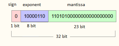
0 01111111101 0000 0000 0000 0000 0000 0000 0000 0000 0000 0000 0000 0000 0000

Where the red part represents the sign, the blue part is for the exponent and the green part represents the mantissa. This explains the strange integer value we saw above as the binary representation of 1070596096 is : 00111111110100000000000000000000 which corresponds to the first 32 bits of 0.25’s binary representation. You can further play with these gdb commands and verify that for instance, by turning our value into -0.25, only the first bit (sign) of its representation is flipped.

Single vs Double precision floats

For now in our C code, we only manipulate double precision floats, coded on 8 bytes (64 bits). Now let’s replace the double variable to a float :

1
2
3
float nbf = 0.25;
nbf = nbf * 0.5;
printf("result: %f\n", nbf);

And re-generate the corresponding assembly code :

1
2
3
4
5
6
7
8
9
10
11
12
13
14
15
16
17
18
19
20
21
22
; floating_points.c:9:     float nbfd = -0.25;
    .loc 1 9 11
    movss	xmm0, DWORD PTR .LC0[rip]	; tmp85,
    movss	DWORD PTR -4[rbp], xmm0	; nbfd, tmp85

; floating_points.c:10:     nbfd = nbfd * 0.5;
    .loc 1 10 10
    movss	xmm1, DWORD PTR -4[rbp]	; tmp87, nbfd
    movss	xmm0, DWORD PTR .LC1[rip]	; tmp88,
    mulss	xmm0, xmm1	; tmp86, tmp87
    movss	DWORD PTR -4[rbp], xmm0	; nbfd, tmp86

; floating_points.c:11:     printf("result: %f\n", nbfd);
    .loc 1 11 5
    pxor	xmm2, xmm2	; _1
    cvtss2sd	xmm2, DWORD PTR -4[rbp]	; _1, nbfd
    movq	rax, xmm2	; _1, _1
    movq	xmm0, rax	;, _1
    lea	rax, .LC2[rip]	; tmp89,
    mov	rdi, rax	;, tmp89
    mov	eax, 1	;,
    call	printf@PLT	;

We can see that the double precision floats operations from the previous code have been replaced by their single precision versions : movsd ➡️ movss and mulss ➡️ mulsd. We also discover a new operation : cvtss2sd that allows to convert a single precision floats to a double precision one. The reason why this instruction appears here is because the printf function only handles as parameters double precision floats 🤷.

We may note 📝 that such operation is not present for integer numbers. Indeed, the floating point representation significantly differs between the single and double precision modes. For integers however, the binary representation is basically the same and the conversion just consists in moving bits from one place to another ↔️.

From integers to floats

One last useful aspect from floats is their conversion from and to integers. Let’s try with a last piece of C code :

1
2
3
int val_int = 42;
double val_double = (double)val_int;
float val_float = (float)val_int;

This compiles to the following assembly instructions :

1
2
3
4
5
6
7
8
9
10
11
12
13
; floating_points.c:17:     int val_int = 42;
    .loc 1 17 9
    mov	DWORD PTR -16[rbp], 42	; val_int,
; floating_points.c:18:     double val_double = (double)val_int;
    .loc 1 18 12
    pxor	xmm0, xmm0	; tmp84
    cvtsi2sd	xmm0, DWORD PTR -16[rbp]	; tmp84, val_int
    movsd	QWORD PTR -8[rbp], xmm0	; val_double, tmp84
; floating_points.c:19:     float val_float = (float)val_int;
    .loc 1 19 11
    pxor	xmm0, xmm0	; tmp85
    cvtsi2ss	xmm0, DWORD PTR -16[rbp]	; tmp85, val_int
    movss	DWORD PTR -12[rbp], xmm0	; val_float, tmp85

We discover here two additional operations : cvtsi2sd and cvtsi2ss. These are the operations that respectively converts integers to single and double precision floats by truncation. By doing the opposite way, we can also identify the operations to convert from floats to integers.

The ASCII Mandelbrot set

Let us now achieve our goal in this chapter : drawing the ASCII Mandelbrot set. We will draw it in the terminal in ASCII, meaning the “pixels” will be represented by text characters. This will be the simplest form of such drawing as no colors or shading will be used.

The Mandelbrot set ? 🤔

The Mandelbrot set is a set of points defined on the complex plane. Drawing this set allows to visualize a complex mathematical object with chaotic borders.

We will draw a grid of characters to represent it in the terminal. Each character of the grid will represent the 2d coordinate of a point in the complex plane. We will define a function that, for each of the point, indicates if it belongs to the Mandelbrot set or not.

In order to avoid spending too much time on the mathematical aspects, we will use the naïve algorithm presented on this page and simply translate it into assembly :

1
2
3
4
5
6
7
8
9
10
11
12
13
14
15
for each pixel (Px, Py) on the screen do
    x0 := scaled x coordinate of pixel (scaled to lie in the Mandelbrot X scale (-2.00, 0.47))
    y0 := scaled y coordinate of pixel (scaled to lie in the Mandelbrot Y scale (-1.12, 1.12))
    x := 0.0
    y := 0.0
    iteration := 0
    max_iteration := 1000
    while (x*x + y*y ≤ 2*2 AND iteration < max_iteration) do
        xtemp := x*x - y*y + x0
        y := 2*x*y + y0
        x := xtemp
        iteration := iteration + 1

    color := palette[iteration]
    plot(Px, Py, color)

In this algorithm, you may realize that the complex numbers are not properly present since their real part x and their imaginary part y are handled separately. This will actually simplify the assembly implementation as complex numbers are not natively present.

We can see that the first step is the computation of the initial points, that are scaled from our grid “pixels” coordinates into the complex plane coordinates. Then, for each initial point, the test consists in studying the convergence of a sequence 🌀 that depends on the coordinates. In this pseudocode, the number of iteration is used to assign a color to the pixel. In our case however, we will simply return a boolean value that indicates if wether the function has converged or not for a given initial value.

The draw_mandelbrot function ✏️

To organize our code, we will proceed similarly to the previous chapter by splitting it into two different functions. We will start by writing a function draw_mandelbrot that iterates over the grid coordinates and print a character that depends on its convergence test :

1
2
3
4
5
6
7
8
9
10
11
12
13
14
15
16
17
18
19
20
21
22
23
24
25
26
27
28
29
30
31
32
33
34
35
36
37
38
39
40
41
42
43
44
45
46
47
48
49
50
51
52
53
54
55
56
57
58
59
60
61
62
63
64
65
66
67
68
69
70
71
72
73
74
75
76
77
78
79
80
81
82
83
84
85
86
87
88
89
90
91
92
93
94
95
96
97
98
99
100
101
102
103
104
; draw the ascii mandelbrot set
; edi: width
; esi: height
draw_mandelbrot:

    push rbp
    mov rbp, rsp

    ; stack allocation
    sub rsp, 40 ; 32 + 8
    ; width: rbp-4, 4 bytes
    ; height: rbp-8, 4 bytes
    ; row index: rbp-12, 4 bytes
    ; col index: rbp-16, 4 bytes
    ; x0 mandelbrot: rbp-24, 8 bytes
    ; y0 mandelbrot: rbp-32, 8 bytes

    ; store the parameters
    mov [rbp-4], edi
    mov [rbp-8], esi

    ; preserving registers
    push rdi
    push rsi
    push rbx

    mov [rbp-12], dword ptr 0
    .L_for_row:

        ; compute y0
        ; [...]

        mov [rbp-16], dword ptr 0
        .L_for_col:

            ; compute x0
            ; [...]

            ; test the point convergence
            ; [...]

            test ax, ax
            jnz .L_if_not_converge

            ; .L_if_converge:

                ; print a star
                mov rax, 1
                mov rdi, 1
                lea rsi, [star_character]
                mov rdx, 1
                syscall

                jmp .L_end_if_converge

            .L_if_not_converge:

                ; printing a space
                mov rax, 1
                mov rdi, 1
                lea rsi, [space_character]
                mov rdx, 1
                syscall

            .L_end_if_converge:

            inc dword ptr [rbp-16]
            mov eax, [rbp-4]
            cmp eax, [rbp-16]
            jne .L_for_col

        ; print a line return
        mov rax, 1
        mov rdi, 1
        lea rsi, [new_line]
        mov rdx, 1
        syscall

        inc dword ptr [rbp-12]
        mov eax, [rbp-8]
        cmp eax, [rbp-12]
        jne .L_for_row

    ; restoring preserved registers
    pop rbx
    pop rsi
    pop rdi

    mov rsp, rbp
    pop rbp

    ret

.data

star_character:
    .word '*'
space_character:
    .word ' '
new_line:
    .word '\n'

; complex plane bounds
; [...]

The function takes as parameters the width and the height of the character grid. Its structure is similar to what we saw in previous chapters : there are two nested loops to iterate over the rows and the columns respectively.

For each coordinate of the grid, the corresponding x0 and y0 values of the complex plane are computed. In this program, we will work with double precision floats. After computing the initial values, the algorithm calls the function that tests the convergence of the point. Depending on the result, either a star character “*” or a blank character “ ” is printed in the terminal. Here for simplicity we perform the printing operation 🖨️ through system calls as we did in the first chapter.

Constants definition

Our first step to compute the function is to add as constants the bounds of the complex plane. The values are taken from the pseucode of the Wikipedia page. They can be defined directly as floating point values the following way :

1
2
3
4
5
6
7
8
9
; complex plane bounds
min_x:
    .double -2.00
max_x:
    .double 0.47
min_y:
    .double -1.12
max_y:
    .double 1.12

We can then implement the computation of the floating point values x0 and y0. Starting with y0, what we need is to convert the column index into a decimal value between 0 and 1. Then, this value can be scaled in order to be lie in the provided bounds ([-1.12, 1.12]).

Computation of x0 and y0

This step requires to simultaneously interact with floating point values and integer values (the column index in the grid height). To convert an integer value into a floating point value, we will used the cvtsi2sd instruction which can be compared to a cast in C. This first part in the code loads the grid coordinate and the grid height as 8 bytes floats in the vector registers and then performs necessary arithmetic operations to scale the value :

1
2
3
4
5
6
7
8
9
10
11
12
13
.L_for_row:

    ; compute y0
    cvtsi2sd xmm1, dword ptr [rbp-12] ; load the row index as a 8 bytes float
    dec dword ptr [rbp-8]
    cvtsi2sd xmm3, dword ptr [rbp-8] ; load the height as a 8 bytes float
    inc dword ptr [rbp-8]
    divsd xmm1, xmm3 ; compute a y position in [0, 1]
    movsd xmm3, [max_y]
    subsd xmm3, [min_y]
    mulsd xmm1, xmm3 ; scale the [0,1] position by (max_y-min-y)
    addsd xmm1, [min_y] ; add min_y to the position
    movsd [rbp-32], xmm1 ; store y0

The computation of x0 is done similarly :

1
2
3
4
5
6
7
8
9
10
11
12
13
.L_for_col:

    ; compute x0
    cvtsi2sd xmm0, dword ptr [rbp-16]
    dec dword ptr [rbp-4]
    cvtsi2sd xmm3, dword ptr [rbp-4]
    inc dword ptr [rbp-4]
    divsd xmm0, xmm3
    movsd xmm3, [max_x]
    subsd xmm3, [min_x]
    mulsd xmm0, xmm3
    addsd xmm0, [min_x]
    movsd [rbp-24], xmm0

📝 Note the as the function contains 2 nested for loops, the computation of the y0 and x0 are not done at the same place. Indeed, as the first loop concerns the rows, it is not necessary to re-compute the y0 index for each iteration on the columns. Since floating point computation is expensive, this can be further optimized by storing the x0 values in an array.

We can already test this first code by calling printf at each column iteration in order to print our the two values x0 and y0. To do so, we will define a string with adequate formatters for floating point double precision values and pass parameters to printf as we saw previously :

1
2
3
4
5
6
7
8
9
10
11
12
13
14
15
16
.L_for_col:

    ; compute x0
    ; [...]

    ; display x0 and y0
    mov eax, 2
    lea rdi, [formatter]
    movsd xmm0, [rbp-24]
    movsd xmm1, [rbp-32]
    call printf

; [...]

formatter:
    .asciz "x0, y0: %f, %f\n"

Here the values of x0 and y0 are taken from the stack memory. You may notice that this time 2 floating point values are passed to printf, hence the value 2 stored in eax.

This code can already be tested to verify that the different values of x0 (in range [-2., 0.47]) and y0 (in range [-1.12, 1.12]) are displayed at each iteration.

The test_convergence function

Now that the main function is in place, it is time to write the convergence function. For each different couple of (x0, y0) values, this function will perform some number of iterations in order to decide if, for the initial values, it converges or not, indicating whether the initial point belongs to the Mandelbrot set.

1
2
3
4
5
6
7
8
9
10
11
12
13
14
15
16
17
18
19
20
21
22
23
24
25
26
27
28
29
30
31
32
33
34
35
36
37
38
39
40
41
42
43
44
45
46
47
48
49
50
51
52
53
54
55
56
57
58
59
60
61
62
63
64
65
66
67
68
69
70
71
72
73
74
75
76
; test if a point converges in the Mandelbrot set
; param x0: xmm0
; param y0: xmm1
; return a boolean in ax
test_convergence:

    push rbp
    mov rbp, rsp

    sub rsp, 56 ; 46 + 10
    ; x0: rbp-8, 8 bytes
    ; y0: rbp-16, 8 bytes
    ; x: rbp-24, 8 bytes
    ; y: rbp-32, 8 bytes
    ; xtemp: rbp-40, 8 bytes
    ; iter, rbp-44, 4 bytes
    ; return flag, rbp-46, 2 bytes

    ; preserving registers
    push rdi
    push rsi
    push rbx

    ; save the parameters x0 and y0
    movsd [rbp-8], xmm0
    movsd [rbp-16], xmm1

    ; init x=0 and y=0
    xorps xmm0, xmm0
    movsd [rbp-24], xmm0
    movsd [rbp-32], xmm0

    ; init the return flag
    xor ax, ax
    mov [rbp-46], ax

    ; init the iter variable
    mov [rbp-44], dword ptr 0

    ; main loop for convergence test
    .L_for_conv:

        ; test the convergence
        ; [...]

        ; .L_convergence_verified:

            mov [rbp-46], word ptr 1
            jmp .L_end_for

        .L_convergence_not_verified:

        ; compute the next iteration
        ; [...]


        ; increase the iteration variable and test for the loop termination
        inc dword ptr [rbp-44]
        mov eax, [max_iteration]
        cmp eax, [rbp-44]
        jne .L_for_conv

    .L_end_for:

    ; set the return flag
    mov ax, [rbp-46]

    ; restoring the preserved registers
    pop rbx
    pop rsi
    pop rdi

    ; returning
    mov rsp, rbp
    pop rbp
    ret

As we previously did, we will define some constants to make the code simplify the code and make it more readable. One integer constant will define the maximum number of iterations : 500. Two other constants define double precision floats that are used in the convergence algorithm : the value 4., to test the convergence, and the value 2. to compute the new iteration :

1
2
3
4
5
6
7
; constants
max_iteration:
    .word 500
double_4_cst:
    .double 4.
double_2_cst:
    .double 2.

Computation of the next iteration x and y

We can now write the code to compute the values of x and y for the next iteration of the convergence test. We will follow the pseudocode with 3 different steps : the computation of a temporary value xtemp, then the computation of the next y value and finally the computation of the new x value.

For the first step, we use simultaneously the two vector registers xmm0 and xmm1 in order to compute x*x and y*y without needing additional memory space :

1
2
3
4
5
6
7
8
9
10
; compute the next iteration

; compute x_temp = x*x-y*y + x0
movsd xmm0, [rbp-24]
mulsd xmm0, [rbp-24] ; xmm0 = x*x
movsd xmm1, [rbp-32]
mulsd xmm1, [rbp-32] ; xmm1 = y*y
subsd xmm0, xmm1 ; xmm0 = x*x-y*y
addsd xmm0, [rbp-8] ; xmm0 = x*x-y*y + x0
movsd [rbp-40], xmm0 ; store x_temp = xmm0 = x*x-y*y + x0

The computation of the new y value then uses only the xmm0 register. This is the place where the constant 2.0 defined earlier is used :

1
2
3
4
5
6
; compute ynext = 2*x*y + y0
movsd xmm0, [double_2_cst] ; xmm0 = 2
mulsd xmm0, [rbp-24] ; xmm0 = 2*x
mulsd xmm0, [rbp-32] ; xmm0 = 2*x*y
addsd xmm0, [rbp-16] ; xmm0 = 2*x*y + y0
movsd [rbp-32], xmm0 ; store y_next = 2*x*y + y0

Finally, the new value of x is copied from the xtemp variable to the stack’s memory. It is necessary to use a temporary xtemp variable since the computation of the new x value depends on the y value :

1
2
3
; compute x_next = xtemp
movsd xmm0, [rbp-40]
movsd [rbp-24], xmm0 ; store x_next = xtemp = x*x-y*y + x0

Testing the convergence

Finally, we can write the convergence test that allows to exit the convergence loop and return a positive answer. The first part consists in computing x*x+y*y, which as done similarly to the computation of the next iteration values. The comparison with the convergence constant 4. is then performed by the (double precision) floating point instruction comisd:

1
2
3
4
5
6
7
8
9
10
11
12
13
14
15
; test for convergence

; computation of x*x + y*y
movsd xmm0, [rbp-24]
mulsd xmm0, xmm0
movsd xmm1, [rbp-32]
mulsd xmm1, xmm1
addsd xmm0, xmm1

; comparison of x*x+y*y and cst. 4.
movsd xmm1, [double_4_cst]
comisd xmm0, xmm1

; branching if the convergence test is not verified
jbe  .L_convergence_not_verified

You will notice that the jbe instruction is used for branching here. Indeed, the comparison instructions for floats set the carry flag in the flags register. According to what we saw in this chapter, the jle instruction would not trigger a jump regarding this flag.

Wrapping it up and testing the result

The last missing part of our code is the call to the test_convergence function in the draw_mandelbrot function :

1
2
3
4
5
6
7
8
9
10
11
12
13
14
15
16
17
18
draw_mandelbrot:

    ; [...]

        mov [rbp-16], dword ptr 0
        .L_for_col:

            ; compute x0
            ; [...]

            ; test the point convergence
            xorps xmm0, xmm0
            xorps xmm1, xmm1
            movsd xmm0, [rbp-24]
            movsd xmm1, [rbp-32]
            call test_convergence

    ; [...]

We can now perform the final test of our code by calling the draw_mandelbrot function from a main. In my implementation, I used a grid of size 80*30 which gives the following result :

1
2
3
4
5
6
7
8
9
10
11
12
13
14
15
16
17
18
19
20
21
22
                                                         ******
                                                         ******
                                                           ***
                                               **  ******************
                                                ***************************
                                            *******************************
                                          * *********************************
                           *    *         ***********************************
                           ***********   ***********************************
                         *************** ***********************************
                     *** *************************************************
                     *** *************************************************
                         *************** ***********************************
                           ***********   ***********************************
                           *    *         ***********************************
                                          * *********************************
                                            *******************************
                                                ***************************
                                               **  ******************
                                                           ***
                                                         ******
                                                         ******

Perfect! We can clearly see the Mandelbrot set here in our terminal! 🤓

What’s next ?

This chapter was the occasion to review several technical points in assembly and understand how floating points variables are handled. The codes from the chapter is available at the followink link. By now, you should be able to implement any type of algorithm that can rely on the stack for its memory. One of the most important thing here is the ability to autonomously debug the program, with gdb for instance. This skill will help understanding more concepts and progress in assembly. The following chapters will focus on applications of these different notions.